

The growing prominence of Einstein and Tableau certainly suggests that analytics, data science, and business intelligence are important to where Salesforce architecture is heading. Statistics are everywhere in Data Science and the principles of statistics underlie Tableau CRM and Einstein Discovery.
With that in mind, the following are some questions about statistics you may be asked in a data science job interview.
As Randy Sherwood states in his Einstein Discovery instructional video:
“It helps to understand the basic statistical concepts we are leveraging to best understand the results. You don’t need to be a data scientist or a statistician to gain further insight on data using Einstein Discovery. However, it helps to be aware of basic statistical concepts to best interpret results”
Being able to answer these interview questions assumes a foundational understanding of descriptive statistics such as mean, mode, median, quartiles, standard deviation, variance, Z-score (Z), and sampling.
I will use an example from a statistics textbook. Assume a survey of 2279 randomly selected adults indicates 422 are Salesforce users. The question is, how reliably does this sample proportion reflect the population of all adults? In this example, we do not know this population proportion. Estimates about the population of all adults can be made with certain confidence levels and confidence intervals, within a certain margin of error.
1. Define confidence interval
Confidence interval is a range of percentage values that, with a stated degree of certainty, includes a known population characteristic. That population characteristic is a mean, proportion, or standard deviation.
Confidence interval is reported as the sample percentage estimate plus or minus some amount, also expressed as a percentage. Confidence interval reports two pieces of information. 1- a range of plausible values for the population parameter, and 2- a confidence level that expresses the probability that a certain sample statistic reflects the population parameter.
2. What does confidence level mean?
Confidence level is a measure, expressed as a percentage, of how certain a sample statistic includes the population parameter.
In statistics, a sample mean, proportion, or standard deviation is a statistic. A population mean, proportion, or standard deviation is a parameter. Confidence level is a probability. It expresses quantitatively the degree of certainty that a sample statistic reflects a population parameter. The applicable statistics and parameters are mean, proportion, or standard deviation.
3. Explain standard error
Standard error is an estimate of standard deviation. It is used when standard deviation of a sample or population is not known, which is the case with the example in this article. It serves as a measure or indication of spread and variability in a data set.
Standard error is a commonly used unit denomination for margin of error. Margin of error can be expressed as either a percentage value, or in terms of how many standard errors it represents. The formula for standard error is the square root of the sample percentage, multiplied by one minus the sample percentage, divided by sample size:

where:
- p is the sample percentage, which is 422/2279 or about 18.5 percent in the example.
- 1 – p = 1 – 422/2279 which is about 81.5 percent in our example
- n = sample size which is 2279 in this example
- The result of this expression is a percentage:
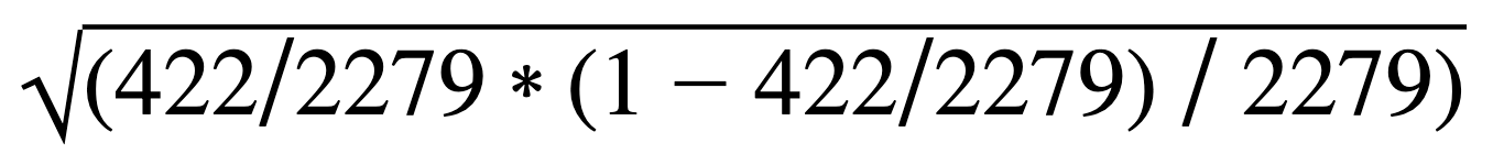
The result is about 0.00814 or 0.814 per cent
4. What is margin of error?
Margin of error is the range of values above and below a sample statistic in a confidence interval. It is a percentage value. It states how many percentage points a test result may differ from the real population value yet still include the actual population statistic. The test result, aka sample statistic, is a mean, proportion, or standard deviation.
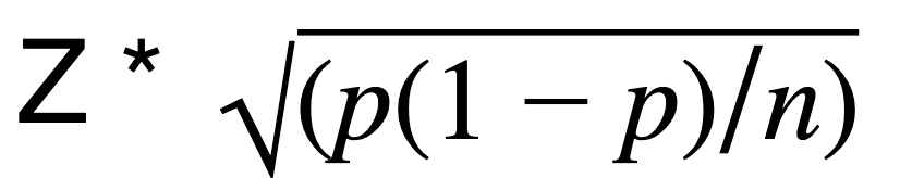
The formula for computing margin of error is the critical Z-value times standard error.
The critical Z value depends on a user’s expectation of desired confidence level. 95% is the most commonly used value. If a 95% confidence level is expected, then the critical Z value is 1.960. Other critical Z values associated with commonly used confidence levels are:
| Confidence Level | Critical Z Value* |
|---|---|
| 90% | 1.645 |
| 95% | 1.960 |
| 99% | 2.576 |
In this example the margin of error for a 90 per cent confidence level is =

which is about 0.013385 or about 1.34 per cent.
In this example the margin of error for a 95 per cent confidence level is =

which is about 0.015947, or about 1.59 per cent.
In this example the margin of error for a 99 per cent confidence level is =

which is about 0.020960, or about 2.10 per cent.
The preceding table of confidence level and critical z values came from the statistics textbook used at a community college where I tutor math. It can be found in any statistics textbook or by searching for confidence level and margin of error.
The critical z value is more pedantically known as ‘Z-Alpha over two’. Find details in any statistics textbook.
Confidence interval, confidence level, standard error, and margin of error; using the example:
The example states 422 of 2279 adults, or about 18.5% of the sample, use Salesforce. The population proportion is not known. Estimates can be made with certain confidence levels and confidence intervals, within a certain margin of error, as to how accurately this 422/2279 sample proportion reflects the population proportion of all adults who use Salesforce.
The margin of error is expressed either in denomination(s) of standard error, or as a percentage. In this example, 18.5 per cent of the sample used Salesforce, plus or minus:
- 1.34 Percent. There is a 90 percent probability that 18.5 percent of all adults, with a 1.34 percent margin of error, use Salesforce. We are 90 percent confident that between 17.2 and 19.8 percent of all adults use Salesforce.
- The confidence level is 90 percent.
- The margin of error is 1.34 percent.
- The confidence interval is 18.5 percent, plus or minus 1.34 percent.
- 1.59 Percent. There is a 95 percent probability that 18.5 percent of all adults, with a 1.59 percent margin of error, use Salesforce. We are 95 percent confident between 16.9 and 20.1 percent of all adults use Salesforce.
- The confidence level is 95 percent.
- The margin of error is 1.59 percent.
- The confidence interval is 18.5 percent, plus or minus 1.59 percent.
- 2.10 Percent. There is a 99 per cent probability that 18.5 per cent of all adults, with a 2.10 per cent margin of error, use Salesforce. We are 99 per cent confident between 16.4 and 20.6 per cent of all adults use Salesforce.
- The confidence level is 99 per cent.
- The margin of error is 2.10 per cent.
- The confidence interval is 18.5 per cent, plus or minus 2.10 per cent.
R script: The preceding computations and calculations are in the following R script. It is here for those of you interested in verifying the math. Paste this command sequence into R and run it from the command line in R Studio. The same figures used in this post will show.
# Sample proportion
p=422/2279
p
# Standard error
se=sqrt(p*(1-p)/2279)
se
# Z score for 95% confidence level
Z=1.960
# Margin of error for 95% confidence level
e=Z*se
e
# Sample proportion +/- one standard error
p+e
p-e
# Sample proportion +/- two standard errors
p+2*e
p-2*e
# Sample proportion +/- three standard errors
p+3*e
p-3*e
# Sample size
Z^2*(p)*(1-p)/e^2
#
# Have R do all the work:
#
if(!require(binom)){install.packages(“binom”)}
library(binom)
binom.confint (x=422, n=2279, conf.level =0.95, method=”all”)
Some of you reading this may come up with figures that differ from what is here, by as much as .05 per cent, depending on whether you are using an online calculator of confidence interval, a scientific calculator such as a TI84, a statistical program such as R, Matlab, or Python; or just doing it by hand. It also depends on the method being used, which may include 1propZint, wilson, bayes, cloglog, or some other method.
5. How do you determine sample size for an experiment?
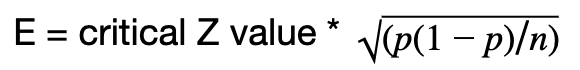
The formula for margin of error is E =
Algebraically isolate n in this expression and the result the formula for sample size:
There are three variables in the resulting expression to consider:
- Z-score (Z)
- sample proportion (p)
- margin of error (E)
When estimating sample size it is important to qualitatively understand the nature, goals, and objectives of the study:
- What is the desired confidence level: 90%? 95%? 99? or …?
- What is the expected population proportion that will exhibit the desired result or effect? Is this portion known or not? If it is not known, use 0.50. This is p in the computation. Using a default value of 0.50 produces the largest possible value of p*(1-p).
- What is the acceptable margin of error? This is E in the computation.
The most commonly used confidence level is 95 percent which corresponds to a Z score of 1.96 standard deviations. Other common confidence levels are cited above in the table of Confidence Level and Critical Z Values
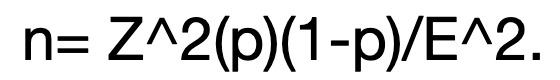
The formula for sample size n is Z^2(p)(1-p)/E^2, where:
- n is the sample size
- Z is the Z-score from the above table
- p is the estimated population proportion. Use 0.5 if it is unknown. This will yield the largest possible value (0.25) of p*(1-p)
- E is the margin of error
Applied to the example problem: 1.96^2 * 422/2279 * (1-422/2279) / 0.0159^2 = 2272
6. What is Hypothesis Testing?
Hypothesis testing is an evidence based decision making process intended to control for the possibility of making mistakes. In many business and scientific contexts decisions are made based on imperfect or limited information. Hypothesis testing is a method for minimizing error when making decisions based on limited or incomplete information.
A hypothesis is a tentative claim about a population made in order to draw out and test its logical or empirical consequences.
In hypothesis testing, a null hypothesis is made about a population, based on a sample. It takes the form of an equality, such as the mean is x, or the proportion is y, or the standard deviation is z. The notation for null hypothesis is Ho, aka H-sub-zero, H_o, or H-naut. Next, an alternate hypothesis is made, representing the approximate complement of the null hypothesis. The alternate hypothesis takes the form of an inequality.
Hypothesis tests can be used to evaluate one of six conditions. These six conditions are inference about population mean, proportion, or standard deviation:
- the mean of a sample
- comparing two sample means
- a sample proportion
- comparing two sample proportions
- standard deviation of a sample
- comparing two standard deviations
Statistical tests are then conducted to determine whether the null hypothesis can be rejected.
Important points about hypothesis tests:
- H_o is always an equality
- In a hypothesis test, the claim is always about the population
- Null hypothesis is the suggestion that nothing of interest is going on. There is no difference between observed and expected data, or no difference between two groups being compared.
- p-values test the hypothesis
7. What is a p-Value?
p-Value is the probability of seeing the same result if the null hypothesis were true. It is the probability that data would be at least as extreme as what would actually be observed if the null hypothesis were true.
The p-Value is a key element of hypothesis testing. It is a percentage value representing the probability of achieving a similar result if the null hypothesis was proven statistically to be true. A small p-Value means there is a higher probability of rejecting the null hypotheses. If the p-value is small there is a difference. Typically “small” is defined as less than 0.05, or five per cent.
8 & 9. What are Type-I and Type-II errors?
Type-I and Type-II errors are mistakes made evaluating a null hypothesis. A Type-I error is when the null hypothesis is true and was rejected. A Type-II error is when the null hypothesis is false and was accepted. Here, a picture is worth a thousand words:
| Accept H_o | Reject H_o | |
|---|---|---|
| H_o is True | Correct Decision | Type-I Error |
| H_o is False | Type-II Error | Correct Decision |
10. How do you detect outliers?
An outlier is a data value in a data set significantly less than the first quartile boundary or significantly greater than the third quartile boundary. It has a quantitative definition. The equation is:
Q1 – 1.5 * IQR, or
Q3 + 1.5 * IQR
The term outlier is often applied to any data value seemingly far from the mean, sample proportion, or median of a data set. This is a reasonable common-sense interpretation of outlier. Statistics textbooks give outliers a quantitative definition and an equation.
To determine if a data value is an outlier:
- Sort the data set
- Identify the median value. This is Q2.
- Identify the median value of the lower half. This is Q1.
- Identify the median value of the upper half. This is Q3.
The data set is now sequenced in four quartiles. Each quartile has about the same number of values, depending on whether there is an even or odd number of values in the data set. Values at the quartile boundaries are called Q1, Q2, and Q3. The absolute value of the difference between data value at Q1 and Q3 is the IQR, or interquartile range. Values in a data set less than Q1 – 1.5 * IQR or greater than Q3 + 1.5 * IQR are outliers.
“Unusual” is a statistics term often used in the context of analyzing outliers. An unusual data value is not the same as an outlier. Unusual also has a standard quantitative definition in Statistics. A value in a data set is ‘unusual’ if it is more than +/- two standard deviations from the mean.
Recap
By way of summary, these definitions and equations answer the original questions in abbreviated form. These are the types of answers that a job interviewer probably wants to hear:

Other principles of statistics in Salesforce Einstein
What is a t-Test? Answering this question in full takes more room than this article will allow. Suffice it to say that t-Test is a statistical probability test applied when sample size is ‘small’ or the standard deviation is not known. This is often the case when trying to determine probabilities using ‘real world’ data from an Einstein dataset. It is relevant to Salesforce because it underlies probability calculations in Einstein Discovery. This is explained in the Randy Sherwood video.
Summary
The predictive features underlying Einstein Discovery make use of standard statistical techniques, many of which are described in this article. Data Scientists who use Einstein Discovery may see questions like this in a job interview.
Check out some of our other Salesforce interview questions below…
- 30 Salesforce Admin Interview Questions & Answers
- 30 Salesforce Developer Interview Questions & Answers
- 50 Most Popular Salesforce Interview Questions & Answers
